Byte-quantized vectors in OpenSearch
Until now, the OpenSearch k-NN plugin has supported the indexing and querying of vectors of type float, with each vector element occupying 4 bytes. This can be expensive in terms of memory and storage, especially for large-scale use cases. Using the new byte vector feature in OpenSearch 2.9, users can reduce memory requirements by a factor of 4 and significantly reduce search latency, with minimal loss in quality (recall).
In this post, we’ll show you how to use byte vectors and how to convert (quantize) 32-bit floats to 8-bit signed integers. We’ll also show you some benchmarking results related to both performance and quality.
Using byte vectors
With byte vectors, each vector element occupies 1 byte (8 bits) and is treated as a signed integer within the range of -128 to 127. This takes advantage of the support for byte vectors in the underlying Lucene engine.
To use a byte vector, set the optional data_type parameter to byte when creating a mapping for an index (the default value of the data_type parameter is float):
PUT test-index
{
  "settings": {
    "index": {
      "knn": true,
      "knn.algo_param.ef_search": 100
    }
  },
  "mappings": {
    "properties": {
      "my_vector1": {
        "type": "knn_vector",
        "dimension": 3,
        "data_type": "byte",
        "method": {
          "name": "hnsw",
          "space_type": "l2",
          "engine": "lucene",
          "parameters": {
            "ef_construction": 128,
            "m": 24
          }
        }
      }
    }
  }
}
Ingestion remains unchanged, but each value in the vector must be within the supported byte range [-128, 127]; otherwise, OpenSearch will return an error:
PUT test-index/_doc/1
{
  "my_vector1": [-126, 28, 127]
}
There is no change in k-NN search. Again, the query vector elements must be within the byte range:
GET test-index/_search
{
  "size": 2,
  "query": {
    "knn": {
      "my_vector1": {
        "vector": [26, -120, 99],
        "k": 2
      }
    }
  }
}
Quantizing float values as bytes
For many applications, existing float vector data can be quantized with little loss in quality.
There are many quantization techniques, such as scalar quantization or product quantization (used in the Faiss engine). The choice of quantization technique depends on the type of data and the k-NN distance metric. It can affect the accuracy of recall, so it is a best practice to run experiments with your own data. Some useful quantization method resources include the following:
- Babak Rokh et al., “A Comprehensive Survey on Model Quantization for Deep Neural Networks in Image Classification”, ACM Transactions on Intelligent Systems Technology, 2023 (in press)
- B. Jacob et al., “Quantization and Training of Neural Networks for Efficient Integer-Arithmetic-Only Inference,” 2018 IEEE/CVF Conference on Computer Vision and Pattern Recognition, Salt Lake City, UT, USA, 2018, pp. 2704-2713, doi: 10.1109/CVPR.2018.00286.
The following section contain Python pseudocode demonstrating a scalar quantization technique suitable for data using Euclidean distance. Euclidean distance is shift invariant; that is, if we shift x and y, then the distance remains the same. Mathematically,
\[\lVert x-y\rVert =\lVert (x-z)-(y-z)\rVert\]Scalar quantization technique for the L2 space type
import numpy as np
# Random dataset (Example to create a random dataset)
dataset = np.random.uniform(-300, 300, (100, 10))
# Random query set (Example to create a random queryset)
queryset = np.random.uniform(-350, 350, (100, 10))
# Number of values
B = 256

# INDEXING:
# Get min and max
dataset_min = np.min(dataset)
dataset_max = np.max(dataset)
# Shift coordinates to be non-negative
dataset -= dataset_min
# Normalize into [0,1]
dataset *= 1. / (dataset_max - dataset_min)
# Bucket into 256 values
dataset = np.floor(dataset * (B-1)) - int(B / 2)

# QUERYING:
# Clip (if queryset range is out of datset range)
queryset = queryset.clip(dataset_min, dataset_max)
# Shift coordinates to be non-negative
queryset -= dataset_min
# Normalize
queryset *= 1. / (dataset_max - dataset_min)
# Bucket into 256 values
queryset = np.floor(queryset * (B - 1)) - int(B / 2)
Scalar quantization technique for the cosinesimilarity space type
Angular datasets using cosine similarity need a different approach because cosine similarity is not shift invariant.
# For Positive Numbers

# INDEXING and QUERYING:

# Get Max of train dataset
max = np.max(dataset)
min = 0
B = 127

# Normalize into [0,1]
val = (val - min) / (max - min)
val = (val * B)

# Get int and fraction values
int_part = floor(val)
frac_part = val - int_part

if 0.5 < frac_part:
 bval = int_part + 1
else:
 bval = int_part

return Byte(bval)
# For Negative Numbers

# INDEXING and QUERYING:

# Get Min of train dataset
min = 0
max = -np.min(dataset)
B = 128

# Normalize into [0,1]
val = (val - min) / (max - min)
val = (val * B)

# Get int and fraction values
int_part = floor(var)
frac_part = val - int_part

if 0.5 < frac_part:
 bval = int_part + 1
else:
 bval = int_part

return Byte(bval)
These are just two simple examples. You will want to evaluate different techniques with your own data to evaluate recall.
Benchmarking results
We ran benchmarking tests on some popular datasets using our k-NN benchmarking perf-tool to compare the quality and performance of byte vectors against float vectors. All the tests were run on the r5.large instance type, which has 2 CPU cores and 16 GB of memory.
SIFT is a feature extraction method that reduces the image content to a set of points used to detect similar patterns in other images. This algorithm is usually related to computer vision applications, including image matching and object detection. A GIST descriptor is a compact representation of an image, which offers advantages such as dimensionality reduction and compatibility with machine learning techniques, making it a valuable choice for approximate nearest neighbor (ANN) tasks in computer vision.
The MNIST dataset is widely used in the field of machine learning and computer vision; it consists of a collection of handwritten digits from 0 to 9 represented as grayscale images of size 28x28 pixels and is a subset of a larger dataset collected by NIST. The GloVe dataset consists of pretrained word vectors generated using the GloVe algorithm. GloVe is an unsupervised learning algorithm used to learn dense vector representations or embeddings for words in a large corpus of text.
Recall and storage results
- Recall@100 – This is the ratio of the top 100 results that were ground truth nearest neighbors. This metric helps you to understand whether you are using a good quantization technique for the dataset.
| Dataset | Dimension of vector | Data size | Number of queries | Training data range | Query data range | Space type | Recall@100 | Index size (GB) | % change in storage | ||
| float | byte | float | byte | ||||||||
| gist-960-euclidean | 960 | 1,000,000 | 1,000 | [ 0.0, 1.48 ] | [ 0.0, 0.729 ] | L2 | 0.99 | 0.96 | 16.5 | 4.2 | 75% |
| sift-128-euclidean | 128 | 1,000,000 | 10,000 | [ 0.0, 218.0 ] | [ 0.0, 184.0 ] | L2 | 0.99 | 0.99 | 1.3 | 0.63 | 52% |
| mnist-784-euclidean | 784 | 60,000 | 10,000 | [ 0.0, 255.0 ] | [ 0.0, 255.0 ] | L2 | 0.99 | 0.99 | 0.38 | 0.12 | 68% |
| glove-50-angular | 50 | 1,183,514 | 10,000 | [ -6.97, 6.51 ] | [ -6.25, 5.85 ] | cosine | 0.99 | 0.94 | 1.3 | 0.35 | 73% |
| glove-100-angular | 100 | 1,183,514 | 10,000 | [ -6.53, 5.96 ] | [ -6.15, 4.22 ] | cosine | 0.99 | 0.92 | 2.6 | 0.62 | 76% |
| glove-200-angular | 200 | 1,183,514 | 10,000 | [ -6.80, 4.61 ] | [ -6.64, 2.72 ] | cosine | 0.99 | 0.77 | 5.1 | 1.1 | 78% |
Indexing and querying results
- Indexing throughput (docs/s) – The number of documents per second that can be ingested.
Document_Cnt / (total_index_time_s + total_refresh_time_s)
Document_Cnt/ (( ingest_took_total)_s + (refresh_index_took_total)_s)
- Query time (ms) – Time per query, summarized as mean, p50, p90, p99.
| Dataset | Dimension of vector | Space type | Indexing throughput (docs/sec) | Query time p50 (ms) | % change in p50 latency | Query time p90 (ms) | % change in p90 latency | Query time p99 (ms) | % change in p99 latency | ||||
| float | byte | float | byte | float | byte | float | byte | ||||||
| gist-960-euclidean | 960 | L2 | 269 | 639 | 711 | 571 | 20% | 1483 | 625 | 58% | 2047 | 697 | 66% |
| sift-128-euclidean | 128 | L2 | 2422 | 2164 | 112 | 67 | 40% | 125 | 75 | 40% | 150 | 96 | 36% |
| mnist-784-euclidean | 784 | L2 | 845 | 935 | 97 | 64 | 34% | 105 | 69 | 34% | 116 | 78 | 32% |
| glove-50-angular | 50 | cosine | 1391 | 1566 | 158 | 89 | 44% | 173 | 96 | 44% | 205 | 119 | 42% |
| glove-100-angular | 100 | cosine | 1014 | 1074 | 252 | 143 | 43% | 291 | 154 | 47% | 324 | 179 | 45% |
| glove-200-angular | 200 | cosine | 640 | 684 | 597 | 260 | 56% | 644 | 279 | 57% | 726 | 316 | 57% |
RSS results
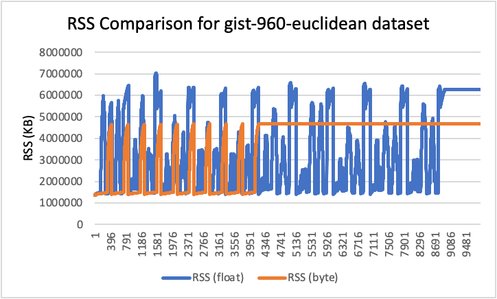
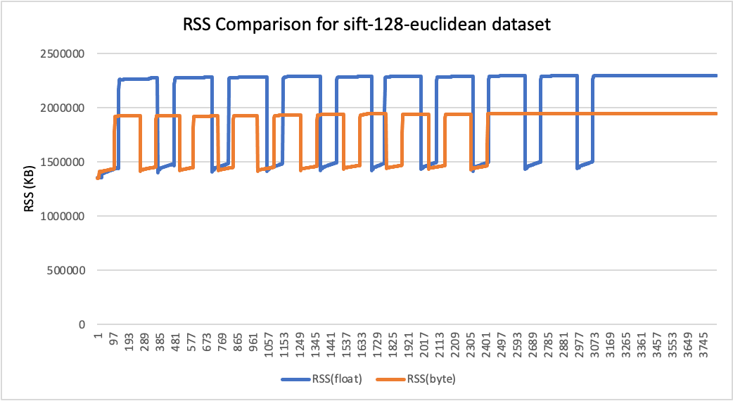
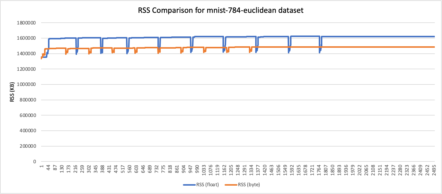
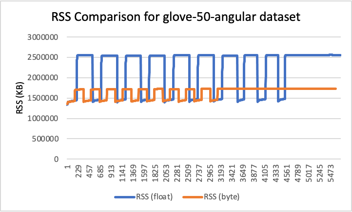
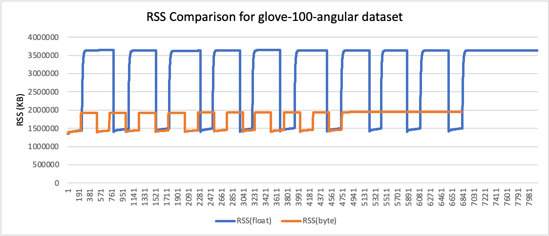
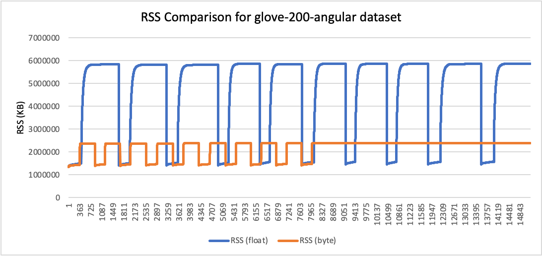
- Peak RSS – The peak of the resident set size obtained by the aggregated sum of RSSAnon (size of resident anonymous memory) and RSSFile (size of resident file mappings).
| Dataset | Dimension of vector | Space type | Peak RSS (GB) | % change in memory | |
| float | byte | ||||
| gist-960-euclidean | 960 | L2 | 6.71 | 4.47 | 33% |
| sift-128-euclidean | 128 | L2 | 2.19 | 1.86 | 15% |
| mnist-784-euclidean | 784 | L2 | 1.55 | 1.42 | 8% |
| glove-50-angular | 50 | cosine | 2.44 | 1.65 | 33% |
| glove-100-angular | 100 | cosine | 3.47 | 1.86 | 47% |
| glove-200-angular | 200 | cosine | 5.6 | 2.27 | 59% |
RSS comparison graphs (in KB)
Analysis
Comparing the benchmarking results, you can see that:
- Using byte vectors rather than 32-bit floats results in a significant reduction in storage and memory usage while also improving indexing throughput and reducing query latency. Precision and recall were not greatly affected, although this will depend on the quantization technique and characteristics of your data.
- Storage usage was reduced by up to 78%, and RAM usage was reduced by up to 59% (for the glove-200-angular dataset).
- Recall values for angular datasets were lower than those of Euclidean datasets. We expect that better quantization techniques would improve recall.
References
- Hervé Jégou, Matthijs Douze, Cordelia Schmid. Product Quantization for Nearest Neighbor Search. IEEE Transactions on Pattern Analysis and Machine Intelligence, 2011, 33 (1), pp.117-128. 10.1109/TPAMI.2010.57 . inria-00514462v2
- Y. LeCun, L. Bottou, Y. Bengio, and P. Haffner. “Gradient-based learning applied to document recognition.” Proceedings of the IEEE, 86(11):2278-2324, November 1998
- Jeffrey Pennington, Richard Socher, and Christopher D. Manning. 2014. GloVe: Global Vectors for Word Representation
